
Modeling Sea Level Rise and Storm Surge Flooding on Long Beach Island, New Jersey
Problem
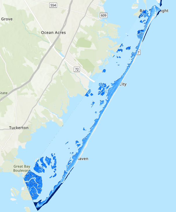
The objective of this study was to model the potential effects of sea level rise upon Long Beach Island, a barrier island off the coast of New Jersey. The island has previously faced severe flooding, including that of 2012 Hurricane Sandy. Using flood models in conjunction with flow models, I aimed to identify areas on the island with the highest risk of storm surge and general sea-level rise flooding. Furthermore, I aimed to characterize the relationship between general socioeconomic risk and flood risk amongst island populations.
Analysis Procedures
Using a 10ft Digital Elevation Model (DEM) from the New Jersey Office of GIS, I generated several initial images using ArcGIS Pro’s watershed analysis tools, including fill, flow direction, flow accumulation, basins, and flow length.
I continued the analysis in GRASS GIS to utilize raster analysis modules, such as r.lake, to model a range of flood scenarios, from mild storm surge to extreme sea-level rise.
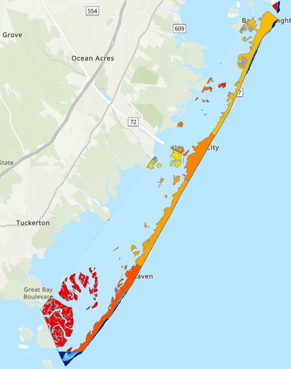
To assess the socioeconomic vulnerability of the area, I overlaid census data with flood models to provide a visual of median income levels compared to flood zones. This analysis highlighted how flood risk disproportionately impacts lower-income communities, where access to mitigation resources is often more limited, offering a clearer picture of the socioeconomic implications of flooding.
Results
Resulting visualizations showed that very few areas of the island are non-susceptible to even relatively low levels of flooding. Points with the least susceptibility include dunes nearby beaches, which are highly mobile and variable year-to-year, and northern areas of the island. Southern portions of the island, including a wildlife reserve, and low-lying main roads are most susceptible. Storm surge and climate change scenarios at any level pose a major threat to life, homes, and businesses, as well as the island’s general longevity and livability. Lower income populations residing in the island’s southern portion are more vulnerable to flood risk.
Reflection
By using GRASS GIS for terrain analysis to run several subsequent hydrologic models, I expanded my technical skills and understanding of several watershed analysis procedures. Integrating census data emphasized how environmental hazards disproportionately affect vulnerable populations, underscoring the importance of interdisciplinary approaches in spatial analysis. Moving forward, I plan to incorporate social vulnerability assessments into my work to ensure that technical solutions account for human health and well-being.
Spatial Autocorrelation of Limited English Proficiency Amongst North Carolina Counties
Problem
The goal of this project was to characterize patterns of Limited English Proficiency (LEP) across North Carolina counties. Using 2015 data from the United States Department of Justice, I aimed to map LEP population density by county, and compute the statistical likelihood that LEP density at the county level occurs by chance.
Analysis Procedures
After joining the dataset with a North Carolina county shapefile in ArcGIS Pro to preserve both spatial geometry and relevant attributes, I loaded this shapefile to R. Using the poly2nb function, I then identified and plotted both rook and queen-type neighbors. After creating a spatial weights matrix (rook) using nb2listw, this was applied to the lag module to compute the spatial lag between LEP density in a county and the LEP density in neighboring counties. With this data, a scatter plot was generated comparing LEP density (x-axis) and neighboring LEP density (y-axis).
Global Moran’s I statistic was computed using the spatial lag input within the lm module along with the associated density field and extracted associated slope information via the output Moran’s I value. Using the moran.test() function, three alternative hypotheses (greater, lower, and two), were assessed to determine the slope’s deviation from the null hypothesis (random distribution). To visualize the likelihood that LEP density values occur by chance, the “greater” null hypothesis (whose output p-value appeared statistically significant) was plotted using moran.mc().
Results
The results of the statistical analysis indicated that LEP density among North Carolina counties was not randomly distributed but instead exhibited significant spatial clustering. The p-values for both the “greater” (0.000002693) and “two” (0.000005387) alternative hypotheses were statistically significant, while the p-value for the “less” hypothesis (1) was not. These findings suggest that counties with high LEP populations tend to be near other counties with similarly high LEP populations rather than being randomly dispersed throughout the state. The Monte Carlo simulation further supported this conclusion, producing a right-skewed distribution that reinforced the presence of spatial autocorrelation.

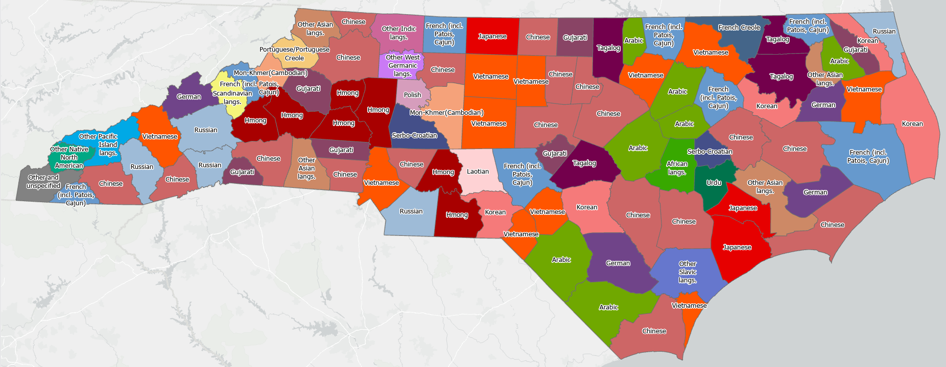
I endeavored to further characterize the nature of LEP populations within North Carolina by finding the most common language spoken aside from English (and Spanish, which is the second-most common language spoken in the vast majority of counties). Additional statistical analysis is needed to further analyze the distribution of common languages spoken amongst North Carolina populations, but an initial output map showing the mode language recorded is shown below.
Reflection
My original intention for this project was to perform a spatial autocorrelation analysis of dialect patterns in the United States. I was more interested in vocabulary differences (for example, soda, pop, coke) than in different languages spoken amongst populations. Finding appropriate data proved more difficult than I expected, so I elected to practice a similar type of analysis using the DOJ LEP data, despite it being slightly dated. I had not used R for several years, so using this language and software reinforced both old and new skills while walking through a method I hope to apply to other datasets in the future. This experience highlighted how data availability can shape the direction of a spatial analysis and reminded me to remain adaptable in my approach. It also reaffirmed my interest in applying spatial methods to cultural and linguistic questions, even in unconventional ways.
